
:)
[DL] Coursera: DL Specialization C1W4A2 본문
Deep Neural Network for Image Classification: Application
import time
import numpy as np
import h5py
import matplotlib.pyplot as plt
import scipy
from PIL import Image
from scipy import ndimage
from dnn_app_utils_v3 import *
from public_tests import *

%matplotlib inline
plt.rcParams['figure.figsize'] = (5.0, 4.0) # set default size of plots
plt.rcParams['image.interpolation'] = 'nearest'
plt.rcParams['image.cmap'] = 'gray'

%load_ext autoreload
%autoreload 2

np.random.seed(1)
Load and Process the Dataset
dataset ("data.h5") :
- cat(1) 또는non-cat(0)로 레이블이 지정된 `m_train` 이미지의 훈련 세트
- 고양이와 고양이가 아닌 것으로 레이블이 지정된 `m_test` 이미지의 테스트 세트.
- 각 이미지의 모양(num_px, num_px, 3)이며, 여기서 3은 3개의 채널(RGB)을 나타낸다.
train_x_orig, train_y, test_x_orig, test_y, classes = load_data()index = 10
plt.imshow(train_x_orig[index])
print ("y = " + str(train_y[0,index]) + ". It's a " + classes[train_y[0,index]].decode("utf-8") + " picture.")y = 0. It's a non-cat picture.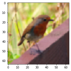
m_train = train_x_orig.shape[0]
num_px = train_x_orig.shape[1]
m_test = test_x_orig.shape[0]

print ("Number of training examples: " + str(m_train))
print ("Number of testing examples: " + str(m_test))
print ("Each image is of size: (" + str(num_px) + ", " + str(num_px) + ", 3)")
print ("train_x_orig shape: " + str(train_x_orig.shape))
print ("train_y shape: " + str(train_y.shape))
print ("test_x_orig shape: " + str(test_x_orig.shape))
print ("test_y shape: " + str(test_y.shape))
Number of training examples: 209
Number of testing examples: 50
Each image is of size: (64, 64, 3)
train_x_orig shape: (209, 64, 64, 3)
train_y shape: (1, 209)
test_x_orig shape: (50, 64, 64, 3)
test_y shape: (1, 50)reshape and standardize the images
# Reshape the training and test examples
train_x_flatten = train_x_orig.reshape(train_x_orig.shape[0], -1).T   # The "-1" makes reshape flatten the remaining dimensions
test_x_flatten = test_x_orig.reshape(test_x_orig.shape[0], -1).T

# Standardize data to have feature values between 0 and 1.
train_x = train_x_flatten/255.
test_x = test_x_flatten/255.

print ("train_x's shape: " + str(train_x.shape))
print ("test_x's shape: " + str(test_x.shape))
train_x's shape: (12288, 209)
test_x's shape: (12288, 50)Model Architecture
two_layer_model
n_x = 12288     # num_px * num_px * 3
n_h = 7
n_y = 1
layers_dims = (n_x, n_h, n_y)
learning_rate = 0.0075
def two_layer_model(X, Y, layers_dims, learning_rate = 0.0075, num_iterations = 3000, print_cost=False):
np.random.seed(1)
grads = {}
costs = []
m = X.shape[1]
(n_x, n_h, n_y) = layers_dims
parameters = initialize_parameters(n_x, n_h, n_y)
W1 = parameters["W1"]
b1 = parameters["b1"]
W2 = parameters["W2"]
b2 = parameters["b2"]
for i in range(0, num_iterations):
A1, cache1 = linear_activation_forward(X, W1, b1, activation="relu")
A2, cache2 = linear_activation_forward(A1, W2, b2, activation="sigmoid")
cost = compute_cost(A2, Y)
# Initializing backward propagation
dA2 = - (np.divide(Y, A2) - np.divide(1 - Y, 1 - A2))
# Backward propagation. Inputs: "dA2, cache2, cache1". Outputs: "dA1, dW2, db2; also dA0 (not used), dW1, db1".
dA1, dW2, db2 = linear_activation_backward(dA2, cache2, activation="sigmoid")
dA0, dW1, db1 = linear_activation_backward(dA1, cache1, activation="relu")
# Set grads['dWl'] to dW1, grads['db1'] to db1, grads['dW2'] to dW2, grads['db2'] to db2
grads['dW1'] = dW1
grads['db1'] = db1
grads['dW2'] = dW2
grads['db2'] = db2
# Update parameters.
parameters = update_parameters(parameters, grads, learning_rate)
# Retrieve W1, b1, W2, b2 from parameters
W1 = parameters["W1"]
b1 = parameters["b1"]
W2 = parameters["W2"]
b2 = parameters["b2"]
# Print the cost every 100 iterations
if print_cost and i % 100 == 0 or i == num_iterations - 1:
print("Cost after iteration {}: {}".format(i, np.squeeze(cost)))
if i % 100 == 0 or i == num_iterations:
costs.append(cost)
return parameters, costs
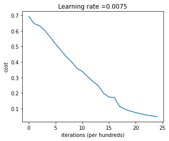
def plot_costs(costs, learning_rate=0.0075):
plt.plot(np.squeeze(costs))
plt.ylabel('cost')
plt.xlabel('iterations (per hundreds)')
plt.title("Learning rate =" + str(learning_rate))
plt.show()parameters, costs = two_layer_model(train_x, train_y, layers_dims = (n_x, n_h, n_y), num_iterations = 2, print_cost=False)
print("Cost after first iteration: " + str(costs[0]))
two_layer_model_test(two_layer_model)Cost after iteration 1: 0.6926114346158595
Cost after first iteration: 0.693049735659989
Cost after iteration 1: 0.6915746967050506
Cost after iteration 1: 0.6915746967050506
Cost after iteration 1: 0.6915746967050506
Cost after iteration 2: 0.6524135179683452Train the model
parameters, costs = two_layer_model(train_x, train_y, layers_dims = (n_x, n_h, n_y), num_iterations = 2500, print_cost=True)
plot_costs(costs, learning_rate)
Cost after iteration 0: 0.693049735659989
Cost after iteration 100: 0.6464320953428849
Cost after iteration 200: 0.6325140647912677
Cost after iteration 300: 0.6015024920354665
Cost after iteration 400: 0.5601966311605747
Cost after iteration 500: 0.5158304772764729
Cost after iteration 600: 0.4754901313943325
Cost after iteration 700: 0.43391631512257495
Cost after iteration 800: 0.4007977536203886
Cost after iteration 900: 0.3580705011323798
Cost after iteration 1000: 0.3394281538366413
Cost after iteration 1100: 0.30527536361962654
Cost after iteration 1200: 0.2749137728213015
Cost after iteration 1300: 0.2468176821061484
Cost after iteration 1400: 0.19850735037466102
Cost after iteration 1500: 0.17448318112556638
Cost after iteration 1600: 0.1708076297809692
Cost after iteration 1700: 0.11306524562164715
Cost after iteration 1800: 0.09629426845937156
Cost after iteration 1900: 0.0834261795972687
Cost after iteration 2000: 0.07439078704319085
Cost after iteration 2100: 0.06630748132267933
Cost after iteration 2200: 0.05919329501038172
Cost after iteration 2300: 0.053361403485605606
Cost after iteration 2400: 0.04855478562877019
Cost after iteration 2499: 0.04421498215868956
predictions_train = predict(train_x, train_y, parameters)Accuracy: 0.9999999999999998predictions_test = predict(test_x, test_y, parameters)Accuracy: 0.72
L_layer_model
layers_dims = [12288, 20, 7, 5, 1] # 4-layerdef L_layer_model(X, Y, layers_dims, learning_rate = 0.0075, num_iterations = 3000, print_cost=False):
np.random.seed(1)
costs = []
# Parameters initialization
parameters = initialize_parameters_deep(layers_dims)
# Loop (gradient descent)
for i in range(0, num_iterations):
# Forward propagation: [LINEAR -> RELU]*(L-1) -> LINEAR -> SIGMOID
AL, caches = L_model_forward(X, parameters)
# Compute cost
cost = compute_cost(AL, Y)
# Backward propagation
grads = L_model_backward(AL, Y, caches)
# Update parameters
parameters = update_parameters(parameters, grads, learning_rate)
# Print the cost every 100 iterations
if print_cost and i % 100 == 0 or i == num_iterations - 1:
print("Cost after iteration {}: {}".format(i, np.squeeze(cost)))
if i % 100 == 0 or i == num_iterations:
costs.append(cost)
return parameters, costsparameters, costs = L_layer_model(train_x, train_y, layers_dims, num_iterations = 1, print_cost = False)
print("Cost after first iteration: " + str(costs[0]))
L_layer_model_test(L_layer_model)Cost after iteration 0: 0.7717493284237686
Cost after first iteration: 0.7717493284237686
Cost after iteration 1: 0.7070709008912569
Cost after iteration 1: 0.7070709008912569
Cost after iteration 1: 0.7070709008912569
Cost after iteration 2: 0.7063462654190897
Train the model
parameters, costs = L_layer_model(train_x, train_y, layers_dims, num_iterations = 2500, print_cost = True)Cost after iteration 0: 0.7717493284237686
Cost after iteration 100: 0.6720534400822914
Cost after iteration 200: 0.6482632048575212
Cost after iteration 300: 0.6115068816101356
Cost after iteration 400: 0.5670473268366111
Cost after iteration 500: 0.5401376634547801
Cost after iteration 600: 0.5279299569455267
Cost after iteration 700: 0.4654773771766851
Cost after iteration 800: 0.369125852495928
Cost after iteration 900: 0.39174697434805344
Cost after iteration 1000: 0.31518698886006163
Cost after iteration 1100: 0.2726998441789385
Cost after iteration 1200: 0.23741853400268137
Cost after iteration 1300: 0.19960120532208644
Cost after iteration 1400: 0.18926300388463307
Cost after iteration 1500: 0.16118854665827753
Cost after iteration 1600: 0.14821389662363316
Cost after iteration 1700: 0.13777487812972944
Cost after iteration 1800: 0.1297401754919012
Cost after iteration 1900: 0.12122535068005211
Cost after iteration 2000: 0.11382060668633713
Cost after iteration 2100: 0.10783928526254133
Cost after iteration 2200: 0.10285466069352679
Cost after iteration 2300: 0.10089745445261786
Cost after iteration 2400: 0.09287821526472398
Cost after iteration 2499: 0.08843994344170202pred_train = predict(train_x, train_y, parameters)Accuracy: 0.9856459330143539pred_test = predict(test_x, test_y, parameters)Accuracy: 0.8Results Analysis
print_mislabeled_images(classes, test_x, test_y, pred_test)
모델이 잘 처리하지 못하는 이미지 유형:
-비정상적인 자세의 고양이
-비슷한 색상의 배경에 고양이가 나타나는 경우
-특이한 고양이 색상 및 종
-카메라 각도
-사진의 밝기
-배율 변화 (고양이가 이미지에서 매우 크거나 작음)
'AI' 카테고리의 다른 글
| [LLM] Large Language Model (3) | 2024.09.13 |
|---|---|
| [DL] Coursera: DL Specialization C2W1A1 (1) | 2024.09.07 |
| [DL] Coursera: DL Specialization C1W4A1 (0) | 2024.08.27 |
| [DL] Coursera: DL Specialization C1W3A1 (0) | 2024.08.16 |
| [DL] Coursera: DL Specialization C1W2A2 (0) | 2024.08.09 |
'AI' Related Articles
more


