[DL Specialization] C1W2A2

고양이를 인식하는 로지스틱 회귀 분류기

import numpy as np
import copy
import matplotlib.pyplot as plt
import h5py
import scipy
from PIL import Image
from scipy import ndimage
from lr_utils import load_dataset
from public_tests import *

%matplotlib inline
%load_ext autoreload
%autoreload 2

 

데이터 개요 및 전처리

# Loading the data (cat/non-cat)
train_set_x_orig, train_set_y, test_set_x_orig, test_set_y, classes = load_dataset()

# Example of a picture
index = 25
plt.imshow(train_set_x_orig[index])
print ("y = " + str(train_set_y[:, index]) + ", it's a '" + classes[np.squeeze(train_set_y[:, index])].decode("utf-8") +  "' picture.")

y = [1], it's a 'cat' picture.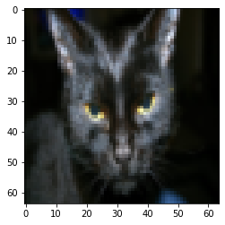

m_train = train_set_x_orig.shape[0]
m_test = test_set_x_orig.shape[0]
num_px = train_set_x_orig.shape[1]

Number of training examples: m_train = 209
Number of testing examples: m_test = 50
Height/Width of each image: num_px = 64
Each image is of size: (64, 64, 3)
train_set_x shape: (209, 64, 64, 3)
train_set_y shape: (1, 209)
test_set_x shape: (50, 64, 64, 3)
test_set_y shape: (1, 50)

train_set_x_flatten = train_set_x_orig.reshape(train_set_x_orig.shape[0], -1).T
test_set_x_flatten = test_set_x_orig.reshape(test_set_x_orig.shape[0], -1).T

train_set_x_flatten shape: (12288, 209)
train_set_y shape: (1, 209)
test_set_x_flatten shape: (12288, 50)
test_set_y shape: (1, 50)

train_set_x = train_set_x_flatten / 255.
test_set_x = test_set_x_flatten / 255.

 

*새로운 데이터 집합의 전처리를 위한 일반적인 단계

1) 문제의 크기와 모양 파악

2) 데이터 집합 재구성

3) 데이터 표준화하기

 

알고리즘 구성

def sigmoid(z):
    s = 1 / (1 + np.exp(-z))
    return s

def initialize_with_zeros(dim):
    w = np.zeros((dim, 1))
    b = 0.0
    return w, b

def propagate(w, b, X, Y):
    m = X.shape[1]
    Z = np.dot(w.T, X) + b
    A = sigmoid(Z)  # A is the sigmoid of Z
    
    cost = (-1 / m) * np.sum(Y * np.log(A) + (1 - Y) * np.log(1 - A))
    
    dw = (1 / m) * np.dot(X, (A - Y).T)
    db = (1 / m) * np.sum(A - Y)
    
    cost = np.squeeze(np.array(cost))

    grads = {"dw": dw,
             "db": db}
    
    return grads, cost

def optimize(w, b, X, Y, num_iterations=100, learning_rate=0.009, print_cost=False):
    
    w = copy.deepcopy(w)
    b = copy.deepcopy(b)
    
    costs = []
    
    for i in range(num_iterations):
        grads, cost = propagate(w, b, X, Y)
        
        # Retrieve derivatives from grads
        dw = grads["dw"]
        db = grads["db"]
        
        w = w - learning_rate * dw
        b = b - learning_rate * db
        
        # Record the costs
        if i % 100 == 0:
            costs.append(cost)
        
            # Print the cost every 100 training iterations
            if print_cost:
                print ("Cost after iteration %i: %f" %(i, cost))
    
    params = {"w": w,
              "b": b}
    
    grads = {"dw": dw,
             "db": db}
    
    return params, grads, costs

def predict(w, b, X):
    m = X.shape[1]
    Y_prediction = np.zeros((1, m))
    w = w.reshape(X.shape[0], 1)
    
    # Compute vector "A" predicting the probabilities of a cat being present in the picture
    A = sigmoid(np.dot(w.T, X) + b)
    
    for i in range(A.shape[1]):
        # Convert probabilities A[0,i] to actual predictions p[0,i]
        if A[0, i] > 0.5:
            Y_prediction[0, i] = 1
        else:
            Y_prediction[0, i] = 0
    
    return Y_prediction

 

def model() : 모델을 학습시키고 예측 작업 수행

X_train, Y_train : 훈련 데이터, 레이블

X_test, Y_test  : 테스트 데이터, 레이블

num_iterations : 반복 횟수

learning_rate : 학습률

print_cost : 비용을 출력할지 여부를 결정

def model(X_train, Y_train, X_test, Y_test, num_iterations=2000, learning_rate=0.5, print_cost=False):
    w, b = initialize_with_zeros(X_train.shape[0])
    
    params, grads, costs = optimize(w, b, X_train, Y_train, num_iterations, learning_rate, print_cost)
    
    # 가중치와 바이어스 업데이트
    w = params["w"]
    b = params["b"]
    
    # 예측 수행
    Y_prediction_test = predict(w, b, X_test)
    Y_prediction_train = predict(w, b, X_train)

    # Print train/test Errors
    if print_cost:
        print("train accuracy: {} %".format(100 - np.mean(np.abs(Y_prediction_train - Y_train)) * 100))
        print("test accuracy: {} %".format(100 - np.mean(np.abs(Y_prediction_test - Y_test)) * 100))

    
    d = {"costs": costs,
         "Y_prediction_test": Y_prediction_test, 
         "Y_prediction_train" : Y_prediction_train, 
         "w" : w, 
         "b" : b,
         "learning_rate" : learning_rate,
         "num_iterations": num_iterations}
    
    return d

 

모델을 학습시키고 예측하는 작업을 수행

logistic_regression_model = model(train_set_x, train_set_y, test_set_x, test_set_y, num_iterations=2000, learning_rate=0.005, print_cost=True)

Cost after iteration 0: 0.693147
Cost after iteration 100: 0.584508
Cost after iteration 200: 0.466949
Cost after iteration 300: 0.376007
Cost after iteration 400: 0.331463
Cost after iteration 500: 0.303273
Cost after iteration 600: 0.279880
Cost after iteration 700: 0.260042
Cost after iteration 800: 0.242941
Cost after iteration 900: 0.228004
Cost after iteration 1000: 0.214820
Cost after iteration 1100: 0.203078
Cost after iteration 1200: 0.192544
Cost after iteration 1300: 0.183033
Cost after iteration 1400: 0.174399
Cost after iteration 1500: 0.166521
Cost after iteration 1600: 0.159305
Cost after iteration 1700: 0.152667
Cost after iteration 1800: 0.146542
Cost after iteration 1900: 0.140872
train accuracy: 99.04306220095694 %
test accuracy: 70.0 %

# Example of a picture that was wrongly classified.
index = 1
plt.imshow(test_set_x[:, index].reshape((num_px, num_px, 3)))
print ("y = " + str(test_set_y[0,index]) + ", you predicted that it is a \"" + classes[int(logistic_regression_model['Y_prediction_test'][0,index])].decode("utf-8") +  "\" picture.")

y = 1, you predicted that it is a "cat" picture.

 

모델 학습 과정에서 cost 변화 시각화

# Plot learning curve (with costs)
costs = np.squeeze(logistic_regression_model['costs'])
plt.plot(costs)
plt.ylabel('cost')
plt.xlabel('iterations (per hundreds)')
plt.title("Learning rate =" + str(logistic_regression_model["learning_rate"]))
plt.show()